
Radio frequency (RF) and wireless design are considered specialist skills within the electronics industry, so usually, only those involved understand the terminology and critical principles. However, embedded designers and hardware engineers increasingly find their development tasks require them to have a basic understanding of RF concepts.
Today, we take always-on connectivity for granted. Wireless communication underpins all our technology, from Bluetooth headsets and cellular smartphones to home media centres and automotive infotainment systems, with ultra-low-power innovations in wireless transceiver design opening up even more potential use cases.
The last two decades have seen wireless connectivity adoption accelerate significantly, so that today wireless connectivity powers personal mobility, delivers freedom from wired connections, and develops communities.
Conveying Information Wirelessly
To fully understand how wireless communication works, designers and engineers need to consider several fundamental concepts. The first is that wireless communication relies on electromagnetic waves, which are synchronised oscillations of electric and magnetic fields propagating through space. The spectrum of electromagnetic radiation is extremely wide, from long-wave radio, microwaves, visible light, and ultraviolet light. The term wavelength, measured in metres, describes the distance between the crests or two corresponding points of an electromagnetic wave (Figure 1), ranging from tens of kilometres (e.g., long wave radio) to tens of nanometres (e.g., infrared). To put it into context, visible light detectable by the human eye ranges from 380 to 700 nanometres.
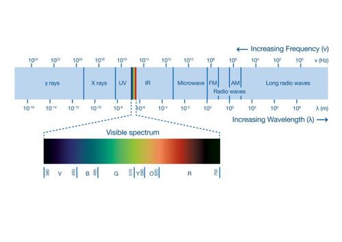
Figure 1: The electromagnetic spectrum ranges from long wave radio waves to x-rays and gamma rays and beyond.
The frequency of electromagnetic waves is measured in cycles per second and called Hertz (Hz). The wavelength is the reciprocal of the frequency.
Usable radio frequencies occupy a significant part of the electromagnetic spectrum (Figure 2) from 30kHz (long wave broadcast stations) to 300GHz (millimetre wavelength bands used for telecommunications and space remote sensing applications).
Radio waves radiate or propagate from a source and, just like light, are impacted by reflections, scattering, and absorption. The nature of propagation varies with frequency and is an essential aspect of radio communication. Understanding how the waves propagate and their paths allow engineers to determine the maximum distance and reliability of communication between two points. Radio waves travelling directly between two points are called ground, direct, or surface waves; over relatively short distances, with no obstacles in between, propagation for these waves is line-of-sight. Radio waves also radiate into the ionosphere, extending the potential distance between a transmitter and a receiver.
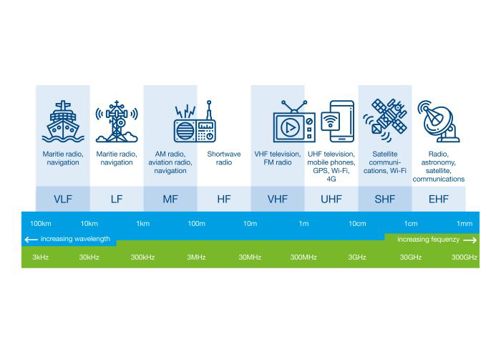
Figure 2: The radio frequency spectrum from very low frequencies (VLF) through to extremely high frequencies (EHF).
The ionosphere comprises different layers: D, E, and F. The layers’ ability to reflect radio waves depends on the sun’s ionisation of the layers, which continually changes with the time of day and season. Short-wave radio waves utilise this form of propagation to cover long distances, but communication can be subject to considerable fading and multiple path reflections. Anyone who has listened to short-wave broadcast stations during the day or night or medium-wave broadcasts at night is probably familiar with fading.
A radio signal consists of a sinusoidal wave of a set frequency called a carrier. The carrier needs modulating to convey any sound or digital data information. There are many different types of modulation in regular use. Amplitude modulation (AM) and frequency modulation (FM) are popular methods used for commercial broadcasting and have been used since the early 1900s. As one might suspect, amplitude modulation changes the amplitude of the carrier signal, whereas frequency modulation maintains a constant amplitude but varies the frequency accordingly to the input sound.
The modulation input is an audio frequency of constant amplitude.
The AM trace highlights how the amplitude of the transmitted signal varies according to the source signal. For FM, the carrier frequency varies instead. Demodulation techniques are employed to extract the original signal from the modulated carrier.
More complex modulation methods used for high-speed data communication include: Binary phase shift keying (BPSK); Orthogonal frequency division multiplex (OFDM) and Quadrature amplitude modulation (QAM)
Basic Receiver Concepts
Figure 3 illustrates the basic functional block diagram of a single-IF stage superheterodyne (superhet) receiver typically used to receive medium-wave and short-wave AM broadcast signals. A mixer and local oscillator (LO) bring the desired RF signal down to an intermediate frequency (IF). By varying the LO, the IF frequency is always the same, simplifying the design of the IF amplifier and filter stages. Traditionally, double mixer/IF stages were used, with IF frequencies of 10.7MHz and 455kHz in many short-wave receivers.
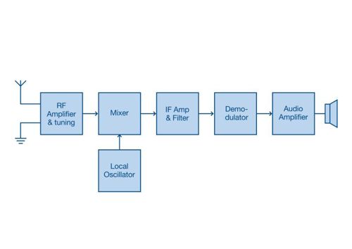
Figure 3: The functional block diagram of a single-stage superhet AM broadcast receiver.
However, a direct conversion or zero IF approach (the LO is set to the desired reception frequency) has now gained popularity, yielding the baseband signal directly out of the mixer ready for demodulation.
A receiver's demodulation and signal processing stages increasingly use software-based digital processing techniques. Software-defined radio (SDR) has become the norm for many complex wireless applications such as cellular base stations, small cells, and secure wireless communications systems.
When dealing with any RF signal, the decibel milliwatt (dBm) is a popular measure of relative signal strength or power output. A dBm is a measure relative to 1mW. As in any decibel measurement, it can also indicate the gain or loss of an amplifier or filter stage. For a receiver, a dBm measurement is typically given as the receiver's sensitivity, the minimum signal strength it can receive. For example, a Wi-Fi module might require a -70dBm signal to operate reliably. Professional short-wave receivers may discern a signal as faint as -100dBm. Satellite navigation receivers are even more sensitive, typically working with signal strengths as low as -150dBm.
The dBm is also used to indicate the gain of an antenna, which is an essential aspect of determining the overall link budget of a wireless communications installation.
Transmitter and Antenna Concepts
Antennas come in all shapes and sizes. In general, the length of an antenna is proportional to the wavelength used and typically either a half-wave or quarter-wave dipole. For very low frequencies, the distances are several kilometres. At the opposite end of the scale, for ultra-high-frequency applications such as Wi-Fi operating at 2.4GHz, a half-wave antenna is just 30mm. To make them even more compact, antenna engineers have some creative shapes that essentially fold up the antenna, making it suitable for PCB fabrication or on a flexible circuit. Figure 4 illustrates an example of a flexible dipole antenna for cellular applications from Linx Technologies.
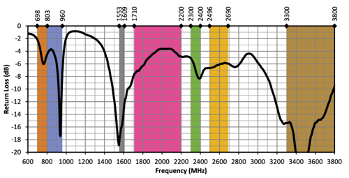
Figure 4: The return loss graph of the Linx Technologies ANT-LPC-FPC-50 antenna.
An antenna impedance must match the impedance of the transmitter's power amplifier output to achieve optimal energy transfer. An impedance of 50 ohms is the universally accepted value for antennas, coaxial cables, and transmitter output stages. If the impedance is mismatched, energy is reflected to the transmitter's power amplifier (PA), which can cause damage if too high. The voltage standing wave ratio (VSWR) indicates how much power is reflected to the transmitter rather than being radiated.
Another way of considering the impedance mismatch of an antenna is by way of a return loss measured in dB. Figure 4 highlights the return loss characteristics of the ANT-LPC-FPC-50 antenna. A lower return loss indicates less power loss due to impedance mismatch.
Two other essential antenna attributes are gain and radiation pattern. The gain is referenced to a theoretical lossless isotropic antenna (radiates uniformly in all directions like a sphere) and expressed in dBi. Some antennas radiate more power in specific directions (i.e., polarisation), so understanding its radiation pattern (Figure 5) will assist engineers in deciding the best mounting location for various use cases. Radiation patterns are normally provided for an antenna as polar charts for each plane.
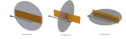
Figure 5: An antenna's radiation pattern involves three different planes.
Achieving a Reliable Wireless Link
To determine if a wireless link over a specific distance is feasible, you need to calculate the link budget. One key factor in calculating the link budget is the free path loss. As a signal is radiated, the geometric spread of the wavefront reduces the power density. The free space path loss calculation determines how much power is received at a distant point. The formula assumes a line-of-sight distance between the transmitter and receiver:
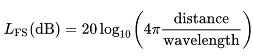
Barriers such as ground features, buildings, and trees increase path loss. Many antenna and wireless manufacturers provide free space path loss calculators on their websites.
Figure 6 illustrates all the factors between a transmitter and a receiver. In the example, the transmitter (Tx) has an output power of +20dBm and is connected to an antenna with a gain of +10dBi. Provision is made for losses in the coaxial cable of -2dBm. On the receiving (Rx) side, a higher-gain antenna yields a gain of +14dBi with cable losses of -2dBm included. The receiver's sensitivity, taken from a datasheet, is quoted as -82dBm. In this example, the path loss over 5km has already been calculated as -114dBm. Will the received signal be sufficient to guarantee a connection? If you add all the highlighted figures (i.e., the link budget), the expected signal is -74dBm, resulting in an 8dBm margin in receiver sensitivity.
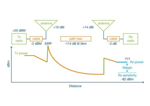
Figure 6: Calculating the link budget is a vital step in determining the reliability of a wireless link between two points.
Wireless Regulatory Compliance
Any radio-frequency-based device may be subject to three different types of regulatory compliance:
Wireless protocol certification – Wireless protocols such as Bluetooth and Wi-Fi may require certification. Modules and wireless transceiver systems-on-chips (SoCs) are certified by the relevant organisations (for example, the Wi-FI Alliance).
Frequency spectrum licencing - As previously mentioned, some wireless communication methods operate within a nationally licensed spectrum (e.g., cellular). Others, such as Bluetooth, do not require a licence to use.
Radio type approvals - In some cases, the national or regional radio regulatory body must approve any wireless module or circuit. The approval process ensures that it causes no unwanted electromagnetic interference to other users and meets all specifications of output power and co-channel interference.
Getting to Grips with Terminology
This article has looked at some basic concepts and terminology surrounding radio frequency and wireless design. Each topic deserves a more in-depth explanation than space permits here, but this should serve as a good starting point for further exploration about this fascinating subject. Although short-wave RF design is little used today, the context helps explain some of the principles covered. Today's wireless engineers typically focus on projects over 100MHz, with relatively short distances. That said, deep space and satellite communication operate over exceptional distances. Some involve high transmitter power and highly directional ultra-high-gain antennas, which are necessary for significant path losses.
Author details: Mark Patrick is a Technical Writer with Mouser Electronics


