
This is called the frequency response of the system. It is represented with a Bode plot. For this, the amplitude response and the phase response are determined from the transfer function of the system and plotted as a graph with the gain and the phase as a function of frequency.
Logarithmic scales are used. The amplitude response is given in decibels, so it is possible to construct complex Bode plots by superposition of simple subplots. If there are several partial transfer functions, the actual multiplication of their amplitude responses is simplified to an addition through the decibel scale. The phase responses can be additively superposed even without the logarithmic scale. Further advantages of the logarithmic representation are the larger frequency range of the plot and the identical relative precision over the entire curve.
Simulation of the Frequency Response with LTspice
The frequency response of an electrical circuit can be simulated with LTspice. With this powerful simulation software for analogue circuits, signals in the time domain can also be transformed to the frequency domain. In addition, small signal analyses and Monte Carlo simulations can be performed. Thanks to its compatibility with SPICE, LTspice can handle numerous electronic components.
To obtain the frequency response of a circuit, or its Bode plot, using LTspice, it helps to start with a simple circuit example. Figure 1 shows a second-order low-pass filter. The input and output nodes were given labels to facilitate the later display of the simulation in the simulation window.
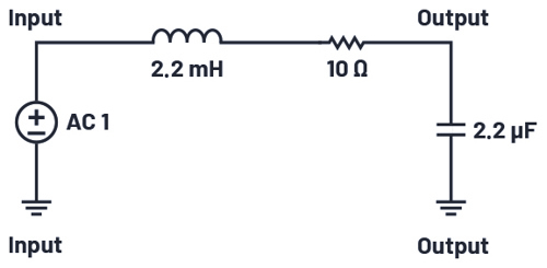
Figure 1. Example of a circuit for a second-order low-pass filter.
The circuit will be stimulated with a sine wave. This requires an AC sweep, which can be found under the AC Analysis tab in the menu Simulate > Edit Simulation Cmd. The simulation parameters are also entered here. The x-axis in a Bode plot should have a logarithmic scale. Under Type of Sweep, the value Decade should be selected. The remaining parameter information should be added as required.
In addition, for the AC analysis, the input voltage with which the circuit should be stimulated should be defined. In the voltage source parameters under menu item Small Signal AC Analysis, the desired amplitude is specified (1V here). Now the actual simulation can be run (Simulate > Run). After the simulation successfully completes, an empty probe editor automatically opens. After the desired node in the circuit (output) has been selected, the amplitude and the phase are displayed as a function of frequency.
The frequency response of a system is yielded from the ratio of the output signal to the input signal; the display still must be adapted slightly. For this, the function must be given as the ratio V(output)/V(input) in the Expression Editor. Now the frequency response of the circuit will correctly show with the amplitude response and the phase response.
Figure 2 shows the frequency response of a second-order low-pass filter as a function of frequency. The amplitude gain is given in decibels on the y-axis on the left, and the phase shift is given in degrees on the y-axis on the right.
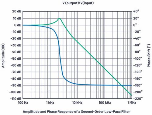
Figure 2. Frequency response as a function of frequency f for a second-order low-pass filter.
To read the exact values from the plot, it is possible to add cursors that you can move along the graph. It is necessary to click on the waveform node title at the top of the graph. If you double-click, you will get two cursors that will give the absolute value at each cursor position and the difference between the two cursor positions in a separate window.
Conclusion
The frequency response of a circuit can be simulated relatively easily with LTspice. The standard Bode plot displayed in LTspice is given as a function of frequency f. A modified method, which is not discussed here, must be used if the plot should be displayed with the angular frequency ω.
Author details: Thomas Brand, Senior Field Applications Engineer, Analog Devices
To contact Thomas Brand use the email address below
To read other Design Tips from Analog Devices follow the link below.


